Machine Learning Models Comparison using Haiti Earthquake Data

Objective

The mission of the project is to provide food aid to people stuck under blue tarps in Haiti due to the earthquake. The data contains pixel images captured from the sites. The pixel correspond to various colors and our goal is to identify the blue tarps. The shape of the data for both the datasets is given below.

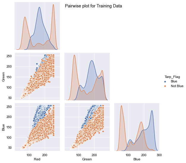
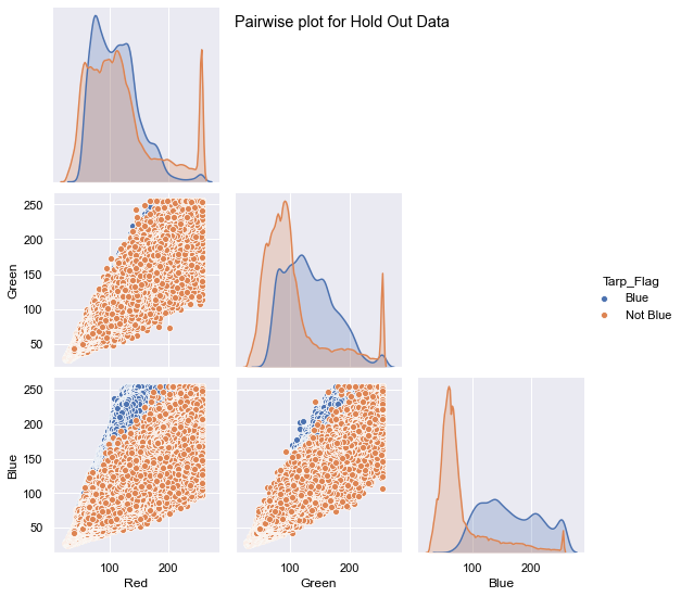
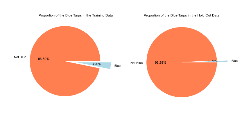
The training data has around ~63k records which contain 3.2% of Blue Tarps and the Hold Out dataset contains ~2million records and has less than 1% blue tarps.

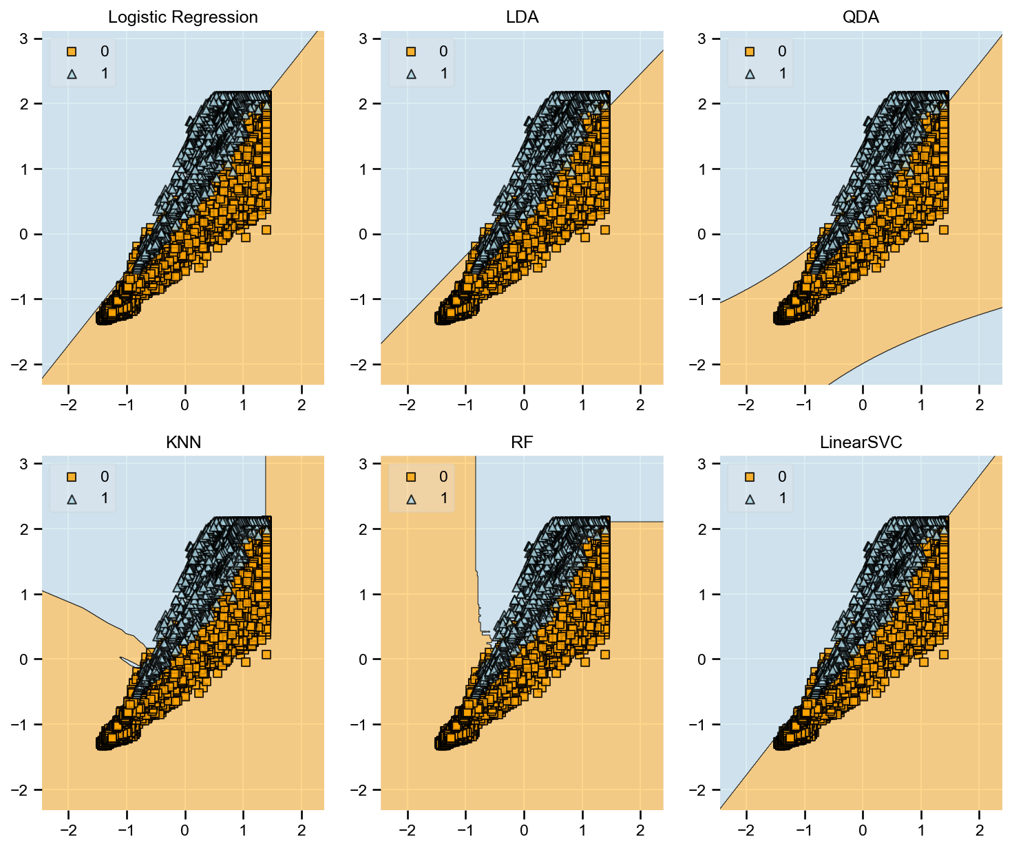
The goal is to compare various machine learning algorithms and discuss the metrics to identify the best model. The list of models being compared are:

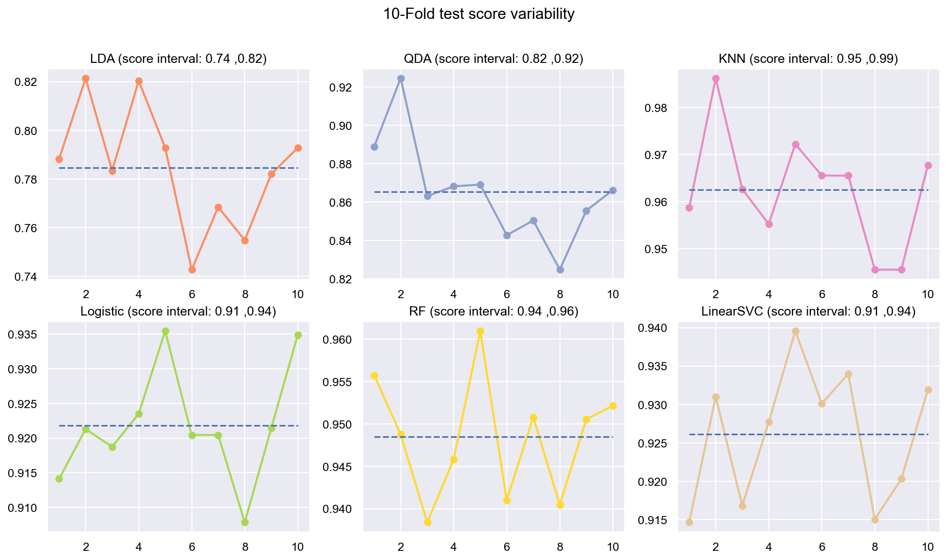
• Linear Discriminant Analysis (LDA)
• Quadratic Discriminant Analysis (QDA)
• K Neighbor Classifier (KNN)
• Logistic Regression (LR)
• Random Forest (RF)
• Linear SVC
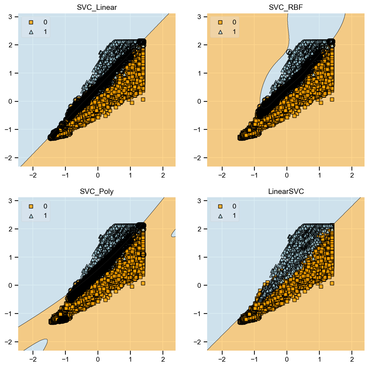
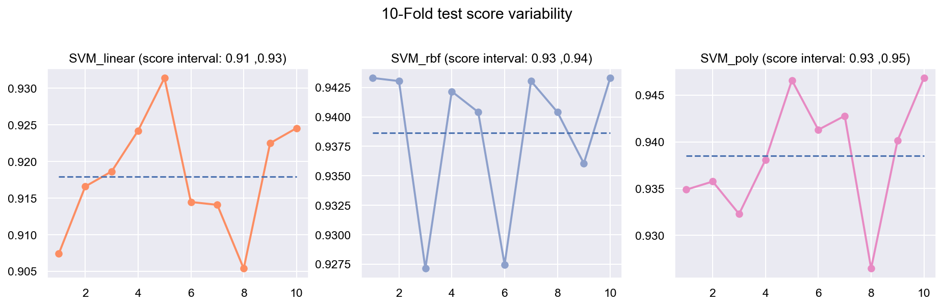
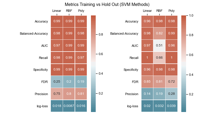
• SVM (Linear Kernel)
• SVM (Radial Kernel)
• SVM (Poly Kernel)

Approach:

Since our main mission is to save lives, we need to identify the Blue Tarps to save the people. However, such missions are limited by resources, time and budget and in many cases, we cannot acheive all the three. It is very crucial to predict the blue tarps accurately as much as predicting the non-blue tarps because we do not want to waste our time and resources on False Positives. Similarly, we also do not want to miss saving lives because of False Negatives.

Some important definitions for terms used throughout the document for quick reference:

True Positives (TP): These are cases in which we predicted YES (Blue Tarps), and they are Blue Tarps.
False Positive (FP): predicted YES, but not Blue Tarps. ("Type I error.")
True Negatives (TN): predicted NO (Not Blue Tarp) and are not
False Negative (FN): predicted NO, but Blue Tarps ("Type II error.")
Accuracy: Overall, how often is the classifier correct

$TP+TN/(TP+FP+TN+FN)$

Balanced Accuracy: Normalizes true positive and true negative predictions by the number of positive and negative samples, respectively, and divides their sum by two

$Balanced Accuracy = ((True Positive Rate + True Negative Rate)/2)$

AUC: Area under the curve. For this document it is the area under the precision-recall curve
Precision: Precision summarizes the fraction of examples assigned the positive class that belong to the positive class

$Precision = TP / (TP + FP)$

Sensitivity or Recall: Recall summarizes how well the positive class was predicted and is the same calculation as sensitivity

$Recall = $TP / (TP + FN)$

F Score: This is a weighted average of the true positive rate (recall) and precision. Special cases of F score based on beta which defines the weight of precision and recall are given below:

• F0.5 - Measure ($beta=0.5$): More weight on precision, less weight on recall
• F1 - Measure ($beta=1.0$): Balance the weight on precision and recall
• F2 - Measure ($beta=2.0$): Less weight on precision, more weight on recall
  
  

False Discovery Rate: The expected proportion of type I errors. A type I error is where you incorrectly reject the null hypothesis; In other words, you get a false positive.

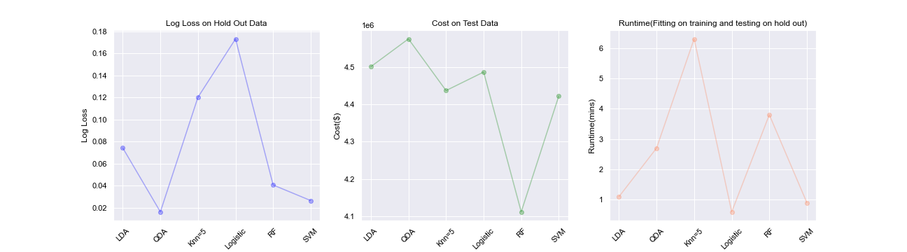
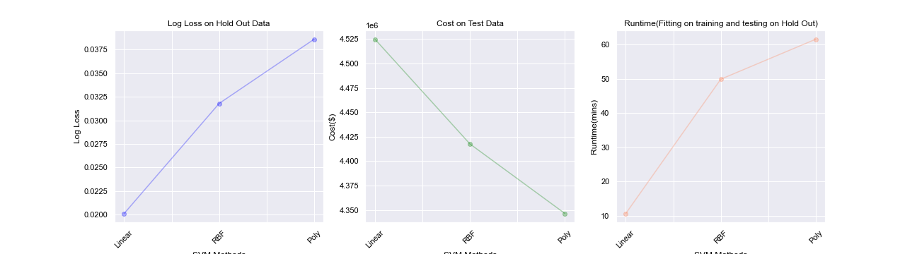
Logarithmic loss (log-loss): Log-loss measures the performance of a classification model where the prediction is a probability value between 0 and 1. Log loss increases as the predicted probability diverge from the actual label. Log loss is a widely used metric for Kaggle competitions. Lower the log-loss value, better are the predictions of the model.

The below measures have been taken to balance the class imbalance, False Positives, False Negatives and to accurately predict True Positives and True Negatives:

• Use Stratified K-FOLD to represent both the classes well in cross-validation
• Use class_weight= ‘balanced’ or equivalent for methods wherever possible to balance both the classes while fitting the data
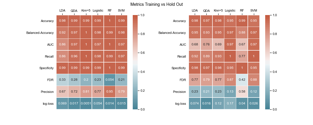
• Use balanced accuracy, precision-recall curve AUC, precision, recall, f-score, log-loss as major metrics to determine the performance of an algorithm.

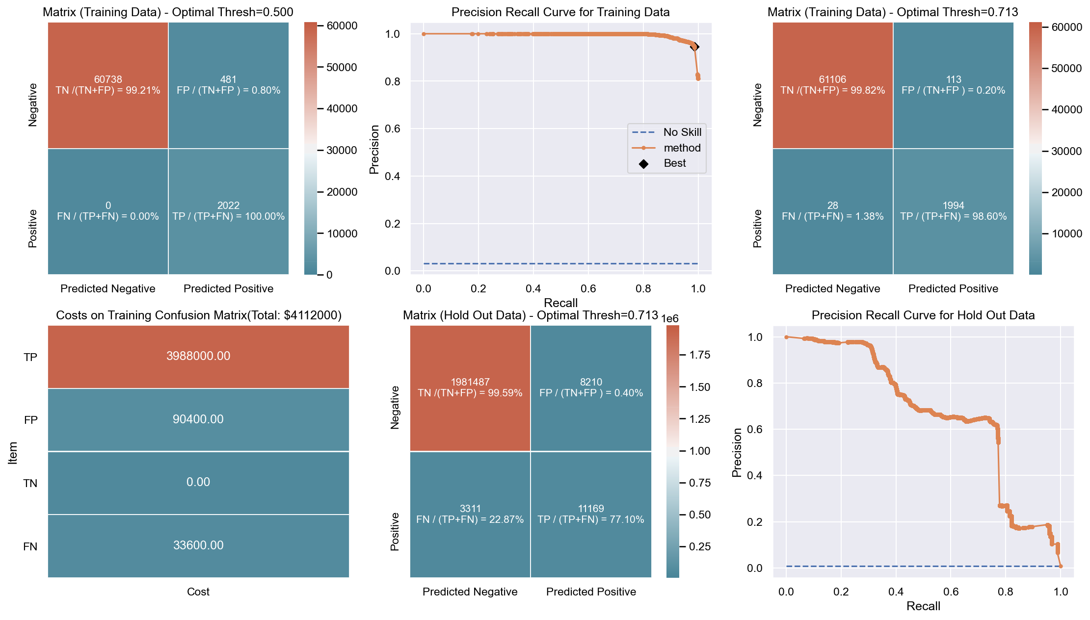
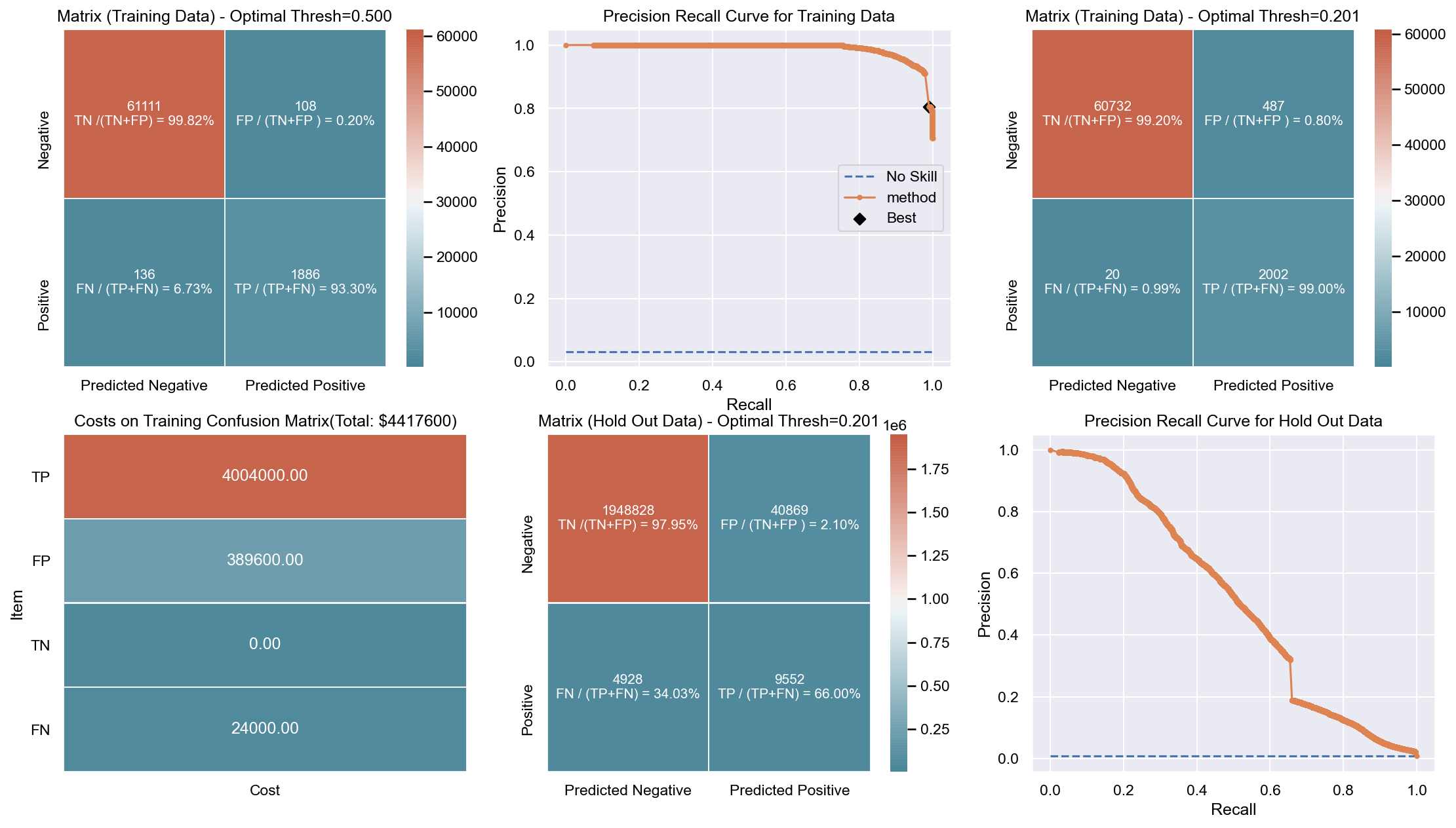
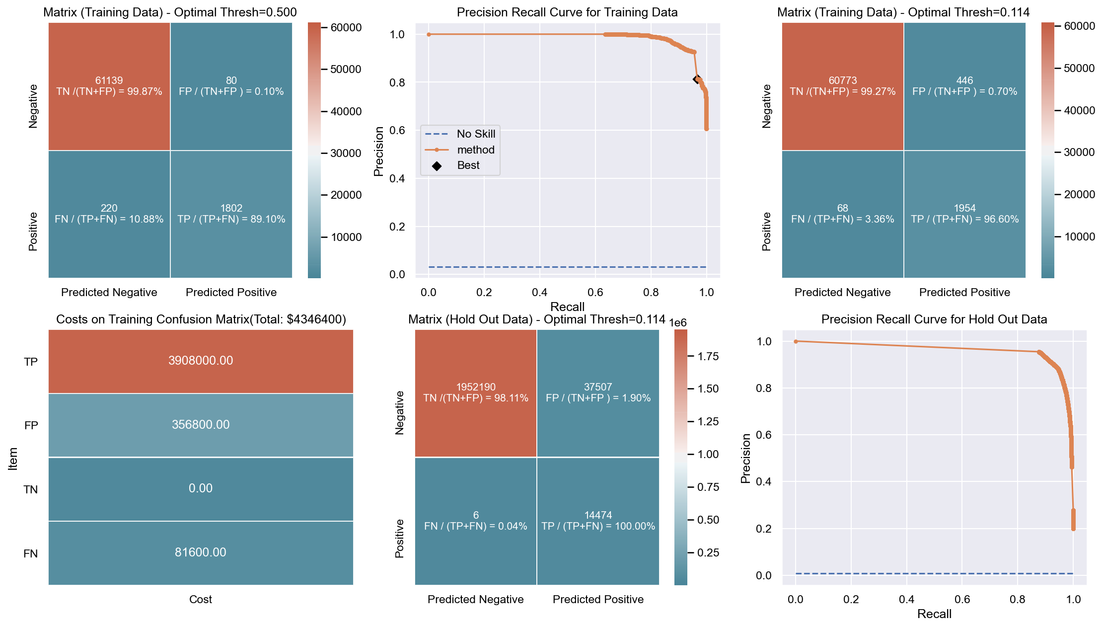
Due to the huge imbalance in data some of the metrics can be mis-leading and especially because we are interested in predicting the positive class which is a minority. The method used to score the cross-validation is ‘fbeta’. Precision and recall matter because in this scenario we also care about resources, time and budget along with prediction capability. Therefore, giving he correct weight to balance precision and recall is critical. To demonstrate the capability of algorithms I decided to use beta as 2 as I personally care more about FN. I created an interactive Jupyter dashboard which can be used to plug in cost values for TP, FP, TN, FN and provide a beta value to see the change and shift in results of costs for various algorithms which can be found here. This dashboard will help the parties make an informed decision by providing the metrics and costs. This can be scaled to pass the algorithm or other parameters which might affect the decisions.

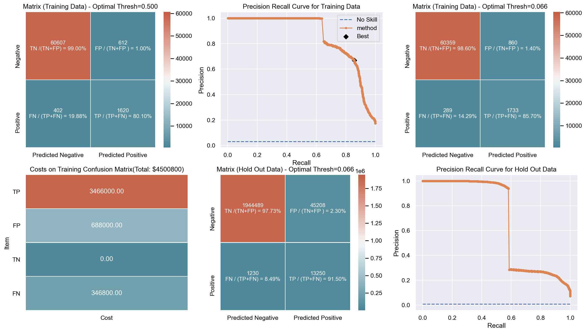
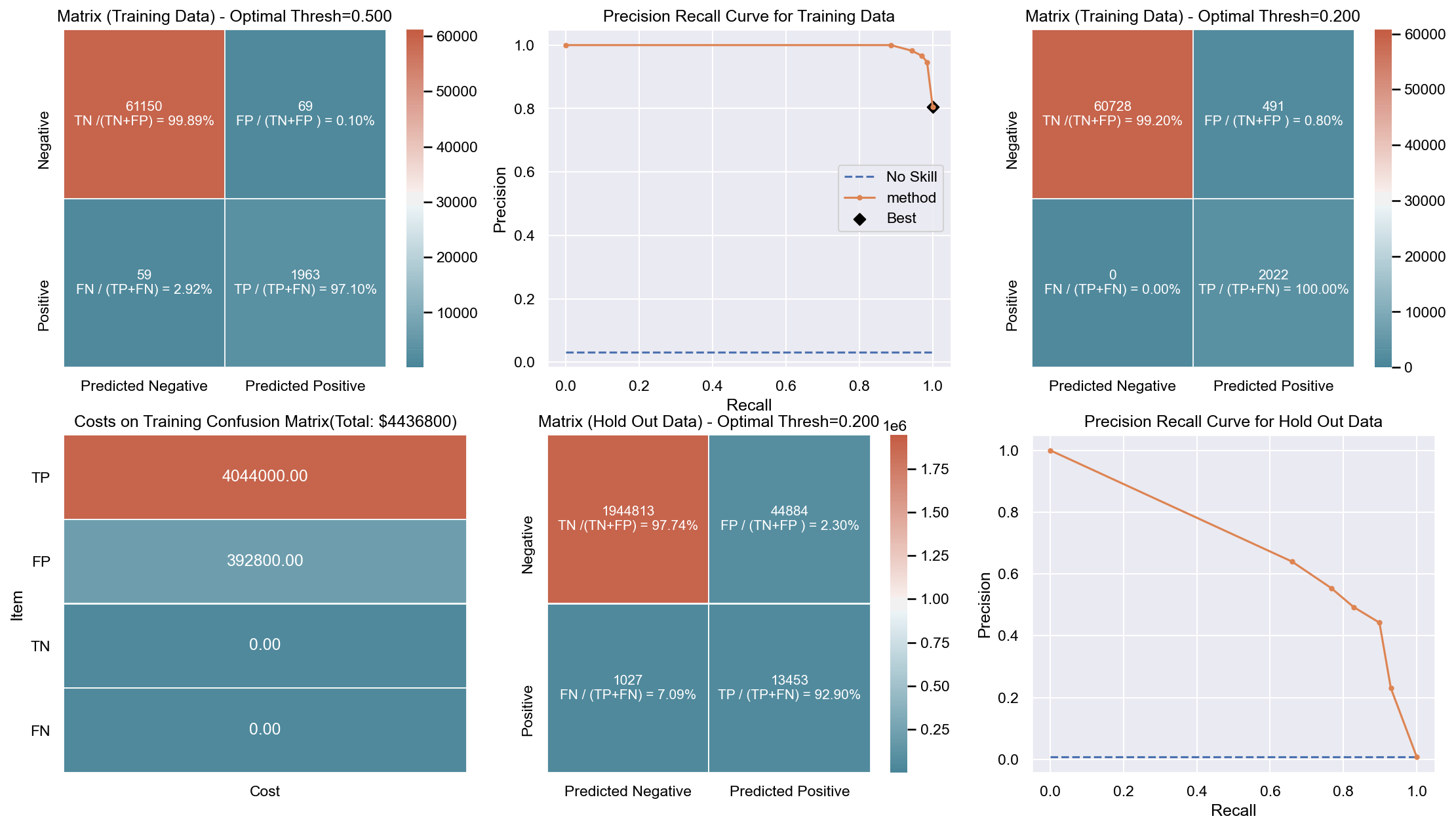
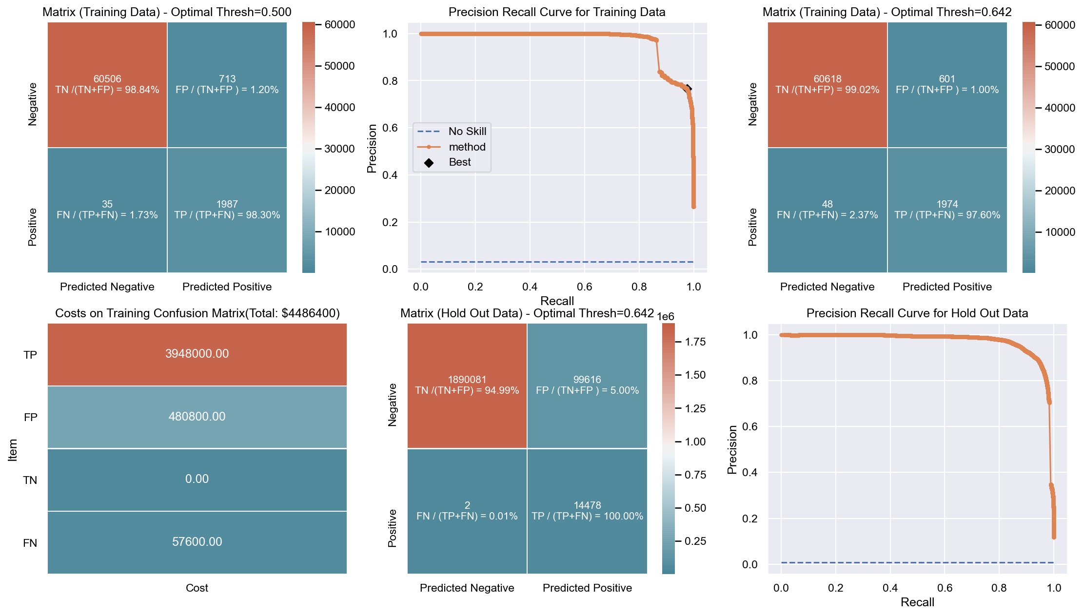
Though it has been challenging to determine the weight for precision and recall, it is hard to ignore the fact that costs will be driving decisions in such a scenario. Therefore, for demonstration purpose I have considered the below hypothetical costs (TP,FP,TN,FN - per person):

Budget: $\$4million$ <br> __TP:__ $\$2000$
FP: $\$800$ <br> __TN:__ $\$0$
FN: $\$1200$

The rational for the costs above are driven by a general cost analysis model. When there is a budget, we assign a cost to everything. Therefore, though the main mission is to save lives it comes with a cost. There is at least cost of employees, fuel and food. Therefore, identifying true positives is more expensive than other categories. Because our mission is still to identify as many Blue Tarps as possible, we have more cost on FN and somewhat less on FP. If we really predict a TN then we do not have any costs as there is no action. To simplify the analysis the goal to stay within $\$4million$, identify as many Blue Tarps as possible. The cost analysis done is just an example to demonstrate an idea of how it can be approached.

Which algorithms appear to be reasonable/good choices for use according to cross-validation?

All the methods perform very well on the training data. K-fold cross validation with 10 folds is performed on each method to choose the best model in each method. The scoring method used for cross validation is f-score with beta as two. Which means FN has more weight than FP. The best model is then used to select the threshold using the f-score with beta as two. The figures shown below are the confusion matrices for each method with the threshold as default at 0.5, precision-recall curve used to select a threshold, a confusion matrix for training data based on the selected threshold, the cost matrix based on the predicted TP, FP, TN and FN, the confusion matrix for hold out data with selected threshold and precision recall curve for hold out data. This is mainly to compute auc.

The AUC is based on the precision and recall curve. We can observe that it is very high for all the methods on the training data. Since the data has huge imbalance in classes and the positive class is a minority, I calculated some extra metrics which will help in determining the performance of an algorithm. I calculated balanced-accuracy and log-loss (Please see definitions in introduction section). I also calculated log-loss, since accuracy is biased towards the larger class and precision/recall need a tradeoff. Purely to measure the performance irrespective of these implications.

|

I also calculated run-time which includes training and predicting on the Hold Out data. We will discuss about this in the following sections. All the methods were under 7-8 mins excpet the SVM kernel methods.The cost based on the training data predictions is lowest for RF because RF’s prediction of True positives is not great. Therefore, we cannot say cost wise RF is the best because we are penalized based on our mission to save people. KNN does well cost wise and good metrics. Logistic Regression and Linear SVM did well cost wise and other metrics. The difference between their costs is is not huge.

Which algorithms actually ended up performing well on the hold-out data?

All the methods did not perform the same on the Hold Out dataset. Linear SVC and SVM linear kernel standout by performing well in almost all metrics and Logistic Regression does well in all except log-loss relatively. All others seem to perform well accuracy wise but not in other metrics. AUC is very low for the hold out data except for Linear SVC and SVM with linear kernel. Though we are doing cross validation and hyper parameter tuning to reduce the over-fitting, some of the methods are not performing well in the metrics we are interested in such as auc. The balanced-accuracy is good for all except RF.

I discussed the reasons why the performance could have reduced on the hold-out data in detail in the next section.

Tuning parameters for Random Forest and SVM methods:

One of the critical steps for performance of an algorithm is selecting the tuning parameters. Especially, for RF and SVM there are many parameters we could consider for tuning. Though we have convenient methods such as GridsearchCV which help with hyper parameter tuning and cross validation it comes with a cost of computational time. The more parameters and range of parameters we tune, it takes longer to tune different combinations. Therefore, it is very important to be strategic in hyper parameter tuning.

Random Forest: Some important parameters which we can tune for Random Forest algorithm are:

• max_depth
• min_sample_split
• max_leaf_nodes
• min_samples_leaf
• n_estimators
• max_sample (bootstrap sample)
• max_features
  

These parameters are important to tune, otherwise RF might over fit the data as many tree algorithms do. Tuning all the parameters above is expensive computationally. Especially in a scenario where you are trying to use it for a disaster relief case, you do not want to spend hours in tuning. With that trade-off, the approach I followed was to do some research on important parameters and understood which might be more suitable with our data. Also, those which improve computational efficiency. I first experimented with everything listed above and finally removed those which did not make a huge difference. I also experimented with value ranges and cut down on the range based on the best model parameters chosen. Eg: if the n_estimators is not going above 100 then I did not include 1000 as a value. This may be problematic if the data changes. However, it is very easy just to tweak the parameters and not affect any other code. I used oob_score=True which helps with run-time and and class_weight and ‘balanced_subsmaple’ to maiantin the balance of classes.

RF specific parameters:

• max_depth: which is very important because if we do not choose a right value then deeper the tree means overfitting of data. In this case it chose 15
• max_samples: the fraction of the original dataset is given to any individual tree. This reduces training time drastically
• max_features: number of max features provided to each tree. I did not consider this one as we have only 3 features in our data and we know that in general RF is good at choosing the important features. This is a critical parameter when we have too many features
  

Decision tree parameters:

• min_samples_split: a parameter that tells the decision tree in a random forest the minimum required number of observations in any given node in order to split it. By increasing the value of the min_sample_split, we can reduce the number of splits that happen in the decision tree and therefore prevent the model from overfitting and we need to be careful in choosing a very high value because RF can start underfitting the data
• n_estimators: number of trees for grouping. This means that choosing many estimators in a random forest model is not the best idea. Although it will not degrade the model, it can save you the computational complexity and prevent the use of a fire extinguisher on your CPU
• max_leaf_nodes: This hyperparameter sets a condition on the splitting of the nodes in the tree and hence restricts the growth of the tree. If after splitting we have more terminal nodes than the specified number of terminal nodes, it will stop the splitting and the tree will not grow further
• min_sample_leaf: the minimum number of samples that should be present in the leaf node after splitting a node. This also helps with overfitting and underfitting.
  

From the above I chose the most important parameters max_depth, n_estimators to begin with. I experimented with the rest and chose min_samples_leaf which was helping with the performance. Since I had the time I was able to experiment. In a time critical situation, we could at least start with max_depth and n_estimators as critical parameters. Overall, these also improved the run-time.

SVM: I compared Linear SVC and SVM with kernels – linear, radial and poly. SVM is a great algorithm but unfortunately does not scale well for larger datasets. It is also computationally expensive. However, on this dataset the linear and poly kernel did pretty well, and linear kernel took much lesser time relatively. The radial kernel had lesser auc and also took a very long time to run (~ 50mins). When I started this project, I was pretty sure that radial would do the best based on the way it works, however it was unable to perform on a large dataset. I tried a small sample and tried to make it work and it still took very long time to run due to tuning parameters. When algorithms like Logistic regression is working seamlessly for this data with very less effort then I could not justify why I would work harder on the others. However, I still researched how that can be improved. There is a group in Taiwan who implemented LinearSVC which is implementation of a Support Vector Classifier. The underlying code is different but for larger datasets and imbalance classes, this seems to work very well compared to SVM implementations. Again, I did not have to work very hard to tune it or use a sub-sample. The run-time is around a minute. I was pretty convinced to choose this over the other SVM methods. However, for demonstration purpose I did use the other SVM methods and computed the metrics.

The tuning parameters for LinearSVC like SVM linear are C and tolerance. For the radial kernel, there is C and gamma and there needs to be a trade-off between both. C is used to control error and gamma is used to give curvature weight of the decision boundary. The interesting thing I have learnt is there is a default value for gamma called scale for gamma. Scale means $1 / (n_features * X.var())$. That seems to have worked the best for the curvature in this case. Therefore, I used that also as part of tuning. For poly, I used gamma and degree. Poly did well but took very long to run. There are few other parameters such as coef_. Since these are computationally expensive, therefore, I experimented to limit the parameters to critical ones and use only those which mattered the most based on the kernel as well.

Confusion Matrices and Precision-Recall Curves for Various methods

Linear Discriminant Analysis

Quadratic Discriminant Analysis

K Nearest Neighbor

Logistic Regression

'

Random Forest

LinearSVC

SVM Linear

SVM RBF

SVM Poly

Compare training and hold out results

The results for training and hold out dataset are mostly compatible. Given the imbalance in the data and increased size, we can see that log-loss increased and the AUC decreased. Based on log-loss LinearSVC and SVM with linear kernel performed great along with other metrics such as balanced-accuracy and AUC. Logistic Regression did well in all except that there is a slight increase in log-loss. SVM with Poly kernel performed equivalent to SVM with linear kernel. However, it takes a very long time to run (~ 50-60min).

Only Random Forest and SVM with rbf kernel have reduced balanced-accuracy, precision-recall auc but the log loss is good for both. Random Forest has tendency to over fit if not properly tuned. The class-imbalance and the linear nature of the data might also be an issue.

If the relationship between the features and the response is well approximated by a linear model then an approach such as linear regression will likely work well, and will outperform a method such as a regression tree that does not exploit this linear structure. If instead there is a highly non-linear and complex relationship between the features and the response as indicated by model (pg 315, ISLR)

We can also look at the decision boundaries graph for comparison methods. These are on the training data. We can see that it does well on the training data and now if we remind ourselves of the shape of the hold-out. If we focus on RF and SVM RBF we can see how there could have been an issue of overfitting. We can say the same about RF as well. Therefore, there was a dip in their precision-recall auc and balanced-accuracy. The LDA and QDA methods did not perform the best because the data doesn't meet the normality assumptions. On the contrary all the linear methods and KNN did well.

Some important steps taken to address the class imbalance were through stratified k-fold, and set class_weight attribute as ‘balanced’. KNN by default considers the classes to be uniform. Performing cross validation keeping the imbalance in mind produced some stable results. We can observe this through the 10-fold variability charts below (please note scale of the graphs. The up and downs can be misleading otherwise). These are f-beta scores of each fold in cross validation and the dotted line is the mean. LDA and QDA have the maximum interval (~0.1) and rest of the methods have an interval of 0.03-0.04. The SVM methods have an interval of 0.01-0.02. This shows that there is not much uncertainty and the models can be considered stable. I experimented using the scoring method as accuracy and balanced-accuracy for the cross validation instead of fbeta. The variability interval for accuracy for ~ 0.001. For balanced-accuracy it was same as the accuracy. The performance of the algorithms dipped slightly for other metrics. Therefore, it is critical to choose a model based on the factors which are important to us and not just based on accuracy which can affect the final performance.

Final Recommendation

The main metric to be considered for this scenario are costs, log-loss, precision-recall auc, balanced-accuracy and run-time. Since there is very clean distinction in performance for balanced-accuracy and auc amongst the methods, I am looking at log-loss, costs and run-time as shown below. Log-loss is a global parameter to give an idea about the algorithm itself without taking into consideration that we care about FN/FP in this situation. Clearly, the Linear SVC model performed well in all aspects and scaled well with large data, imbalance in classes, run-time and costs. However, I am a little hesitant to pick that as the best model since there is not much literature or examples of it. In general, I also know that SVM does not scale well for larger data. It is ideal for high dimensional spaces. Therefore, I am also hesitant to say SVM with Linear kernel is the best algorithm. Purely by metrics (including log-loss) both algorithms stand-out. However, I would still choose Logistic Regression over both algorithms because I understand it well and I can explain the results better and is also known to be robust. It also required least effort and still performed very well. Logistic regression based on all the metrics did well on both training and hold out. The difference in costs between Logistic Regression and LinearSVM is very low. Why go with a more complicated model when logistic is doing so well. If class imbalance was not an issue, then RF was next in the line with very low costs. LDA and QDA as assumed did not do well and we can say that the data did not meet the normality assumption and therefore Logistic had an edge over both.

If we had real costs, we could have made the decision based on costs. The mock cost matrix for each method by TP, FP, TN and FN is given here.

Relevance of the metrics

Accuracy, ROC-AUC, FDR, Specificity are most used and generally good metrics to measure the performance of an algorithm. However, all these metrics emphasize on the larger class and can be misleading for dataset which has class imbalance like the data we are using. Therefore, it is not ideal to choose a best algorithm based on these metrics. Consider a sample with 97 negative and 3 positive values. Classifying all values as negative in this case gives 0.97 accuracy score but we may be more interested in the positive class prediction which is not clear through this metric. ROC is sensitive to the class-imbalance issue, meaning that it favors the class with larger population solely because of its higher population. It is biased towards the larger population when it comes to classification/prediction. This is problematic in such scenarios where we are interested I the positive class which is a minority.

We saw how we can address the imbalance issue for cross validation in the second section. For metrics we can use balanced-accuracy and log-loss. Since we not only care about TP but also care about FN and FP we can also consider the precision, recall, precision-recall curve and auc. Balanced-Accuracy (see definition in objective) can be used instead of accuracy so that it gives a better representative metric of both classes. Since we care about both FN and FP it is hard to decide based on precision and recall metrics since they always have a trade-off. In such cases we can use the precision-recall auc and log-loss to help us choose the best algorithm. Log loss is a widely used metric for Kaggle competitions but is a golbal metric. Lower the log-loss value, better are the predictions of the model.

The other very critical metrics are cost and run-time. As discussed in the first sectiob, SVM with kernels seem to take very long time to run but all other algorithms considerably take very less time. KNN takes the highest excluding the SVM Kernel methods. Costs vary based on what is important to us. In this case though an algorithm has good accuracy for TP, that may be more expensive and at the same time False Negatives are also crucial for our mission. Logistic has a kind of balance between performance and cost.

Future consdierations

‘No Free Lunch’ is truly the main take away for many aspects of this whole exercise. Not only for choosing a statistical method, but for choosing tuning parameters, scoring methods, metrics, understanding various attributes in methods and their significance. The software packages in sci-kit learn are very convenient to use, however it is no good if we do not understand the requirements at hand and methodology of the statistical methods and their significance.

Run time was very frustrating for RF and SVM kernel methods. Some of the important attributes such as n_jobs are critical to allocate threads for the process, oob_score=true for RF improves run-time. Scaling the data is critical for SVM methods. There are convenient methods such as GridsearchCV which can make parameter tuning pretty easy and smooth, however it is critical to understand what parameters to tune, what they mean, how to improve run-time, when and how to scale data. Class_weight is an attribute to specify the class imbalance and the pipeline package can be used to scale the data during cross validation and preventing information leakage to the test data. There is a package called SMOTE and imblearn which help with splitting data using weights. This was challenging to compute the right weights and was risky of over and under representation. There is more learning opportunity here. There are also different cross-validation methods such as randomized search and the grid search. Depending on our usecase both can be considered because randomized search may improve run-time but Gridsearch provides more accuracy. For Gridsearch it is important to pick the most important parameters as it can be computationally expensive. It is crucial to know how to best use computational rsources and manage the run-time.

Code

#### Libraries
# imports and setup
##https://stackoverflow.com/questions/18380168/center-output-plots-in-the-notebook/18401835
from IPython.display import HTML
#IPython.Cell.options_default.cm_config.lineNumbers = False;
import IPython.core.display as di
from IPython.display import Image
import os
import re
import random
import numpy as np
import pandas as pd
import seaborn as sns
#import swifter
import warnings
import time# to measure runtime of the algorithms
import itertools
import statistics as stat
import matplotlib.pyplot as plt
import matplotlib.gridspec as gridspec
from matplotlib.colors import ListedColormap
from sklearn.linear_model import LogisticRegression
from sklearn.metrics import confusion_matrix, accuracy_score, auc, make_scorer, recall_score, precision_score,plot_confusion_matrix, f1_score, fbeta_score, plot_roc_curve, precision_recall_curve,plot_precision_recall_curve,average_precision_score, log_loss
from sklearn.discriminant_analysis import LinearDiscriminantAnalysis, QuadraticDiscriminantAnalysis
from sklearn.neighbors import KNeighborsClassifier
from sklearn.model_selection import train_test_split, cross_val_score, KFold, LeaveOneOut, RepeatedKFold, StratifiedKFold, GridSearchCV, RandomizedSearchCV, StratifiedShuffleSplit, cross_val_predict, learning_curve, validation_curve 
from sklearn import preprocessing
from sklearn.calibration import CalibratedClassifierCV
from sklearn.ensemble import RandomForestClassifier
from sklearn.svm import SVC, LinearSVC
from sklearn.pipeline import Pipeline
from mlxtend.plotting import plot_decision_regions
from sklearn.cluster import KMeans

sns.set() # wil lcreate pretty matplots
%matplotlib inline
#global format settigns for plots
plt.rcParams['font.sans-serif'] = 'Arial'
plt.rcParams['font.family'] = 'sans-serif'
plt.rcParams['text.color'] = '#000000'
plt.rcParams['axes.labelcolor']= '#000000'
plt.rcParams['xtick.color'] = '#000000'
plt.rcParams['ytick.color'] = '#000000'
plt.rcParams['font.size']=12
warnings.filterwarnings('ignore')
pd.set_option('precision', 3) # number precision for pandas
pd.set_option('display.max_rows', 12)
pd.set_option('display.float_format', '{:20,.3f}'.format) # get rid of scientific notation

#### EDA Functions
#Reusable function EDA
def calcProportion(dataset):
    #saving training data proportions by class in a temporary dataframe
    tempdf=pd.DataFrame(index=dataset.Tarp_Flag.unique())
    #tempdf.set_index(0)
    tempdf['Proportion'] = 0
    tempdf["Proportion"] = tempdf["Proportion"].astype(float)
    tempdf['Proportion']['Not Blue']= round((dataset.Tarp_Flag[dataset.Tarp_Flag=='Not Blue'].count()/len(dataset))*100,2)
    tempdf['Proportion']['Blue']= round((dataset.Tarp_Flag[dataset.Tarp_Flag=='Blue'].count()/len(dataset))*100,2) 
    return tempdf

##https://www.dataforeverybody.com/matplotlib-seaborn-pie-charts/
def subplotProportion(plt,tempdf1,tempdf2):
    f, axs = plt.subplots(1, 2,figsize=(12,6));#figsize=(10,6)
    axs[0].pie(x=tempdf1['Proportion'],autopct="%1.2f%%",labels=tempdf1.index,explode=(0.3,0),colors=['#FF7F50','Lightblue'])
    axs[0].set_title("Proportion of the Blue Tarps in the Training Data");
    axs[1].pie(x=tempdf2['Proportion'],autopct="%1.2f%%",labels=tempdf2.index,explode=(0.3,0),colors=['Lightblue','#FF7F50'])
    axs[1].set_title("Proportion of the Blue Tarps in the Hold Out Data");
    return plt

#### Cost Analysis Functions
#https://www.kaggle.com/badolar/using-cost-benefit-matrix-with-confusion-matrix
#https://www.kdnuggets.com/2018/10/confusion-matrices-quantify-cost-being-wrong.html
#https://www.educba.com/cost-benefit-analysis-formula/
def dataForCostAnalysis(TP,FP,TN,FN):
    df = pd.DataFrame({'TP':[TP],'FP':[FP],'TN':[TN], 'FN':[FN]})
    return df

def costAnalysis(cost_data,cost_list,method,threshold):
    data= {'Item': ['TP', 'FP', 'TN', 'FN']}
    cost_mat = pd.DataFrame(data)
    cost_mat['Cost per Person($)'] = cost_list
    cost_mat['Method & Threshold'] = str(method)+'& thresh='+str(threshold)
    cost_mat['Value'] = 0
    cost_mat.loc[0,'Value'] = cost_data['TP'].values; cost_mat.loc[1,'Value'] = cost_data['FP'].values 
    cost_mat.loc[2,'Value'] = cost_data['TN'].values; cost_mat.loc[3,'Value'] = cost_data['FN'].values
    cost_mat = cost_mat.set_index('Item')
    cost_mat['Cost']=cost_mat['Cost per Person($)']*cost_mat['Value']
    return cost_mat

#### Calculate Confusion Matrix, Optimal Threshold and other Metrics (used in predictBlueTarp)
# Reusable functions which are called in the predictBlueTarp function.
# apply threshold to positive probabilities to create labels
def to_labels(pos_probs, threshold):
	return (pos_probs > threshold).astype('int')

#computes optimal threshold based on f1 score. Called from callPrecision_Recall_Curve
def getoptimalThreshold(ax, precision, recall,thresholds, probs,y_train,beta):
    #the function creates a f1 score for the data using al lthe thresholds
    scores_t = [fbeta_score(y_train, to_labels(probs, t),beta=beta) for t in thresholds]
    # get index of best threshold with max score
    ix = np.argmax(scores_t)
    #print('\nBeta=%.2f, Best Threshold=%.3f, F-Score=%.3f' % (beta, thresholds[ix], scores_t[ix]))
    # calculate the no skill line as the proportion of the positive class
    no_skill = len(y_train[y_train==1]) / len(y_train)
    # plot the no skill precision-recall curve
    ax.plot([0, 1], [no_skill, no_skill], linestyle='--', label='No Skill')
    # plot the model precision-recall curve
    ax.plot(recall, precision, marker='.', label='method')
    ax.scatter(recall[ix], precision[ix], marker='D', color='black', label='Best')
    # axis labels
    ax.set_title('Precision Recall Curve for Training Data')
    ax.set_xlabel('Recall')
    ax.set_ylabel('Precision')
    # show the legend
    ax.legend()
    return thresholds[ix]


# https://machinelearningmastery.com/threshold-moving-for-imbalanced-classification/
# Function called to plot ROC and compute optimal threshold 
# Also calls getOptimalThreshold and returns it
def callPrecision_Recall_Curve(ax, fit,X,y,beta):
    y_pred = fit.predict_proba(X)
    # keep probabilities for the positive outcome only
    y_pred = y_pred[:,1]
    precision, recall, thresholds = precision_recall_curve(y, y_pred)
    best_thresh = getoptimalThreshold(ax,precision,recall,thresholds,y_pred,y,beta)
    return best_thresh

#Mainly used to fill the final table of metrics exactly as asked and plot the confusion matrix(cm) where required
#takes the best estimator and any x and y values alogn with a threshold to compute the metrics and cm. used in exploreConfusionMatrix function
#https://github.com/wcipriano/pretty-print-confusion-matrix
#https://matplotlib.org/3.1.1/tutorials/colors/colormaps.html
def getClassificationMetrics(ax,dataset,fit,X,y,y_pred,threshold):
    #compute predicted probabilities
    pred_prob = fit.predict_proba(X)
    #compute log-loass as an extra metric
    l_loss = log_loss(y, pred_prob)
    #keep probabilities for the positive outcome only
    pred_prob = pred_prob[:,1]
    CM = confusion_matrix(y,y_pred)
    TN = CM[0][0]; FN = CM[1][0] ; TP = CM[1][1]; FP = CM[0][1]
    Population = TN+FN+TP+FP
    Accuracy   = round( (TP+TN) / Population,4)
    Recall     = round( TP / (TP+FN),3 )
    FPR        = round( FP / (TN+FP),3 )
    Specificity = 1-FPR
    FDR        = round( FP / (TP+FP),3 )
    Precision  = round( TP / (TP+FP),3 )
    TNR = round(TN/(TN+FP),3)
    b_accuracy   = (Recall+TNR)/2
    #precision and recall arrays to calcualte the precision and recall auc
    precision, recall, _ = precision_recall_curve(y, pred_prob);
    #calcualting precision and recall auc and not roc_auc - very important
    auc_score = round(auc(recall,precision),4)
    if(dataset=='train'): plt.title("Matrix (Training Data) - Optimal Thresh=%.3f" %threshold)
    else: plt.title("Matrix (Hold Out Data) - Optimal Thresh=%.3f" %threshold)
    #get values from the confusion matrix inbuilt function and use it in a seaborn plot to make it look pretty
    group_counts = ["{0:0.0f}".format(value) for value in CM.flatten()]
    group_percentages = ["TN /(TN+FP) = {0:.2%}".format(TN/(TN+FP)), "FP / (TN+FP ) = {0:.2%}".format(FPR), "FN / (TP+FN) = {0:.2%}".format(FN/(TP+FN)), \
        "TP / (TP+FN) = {0:.2%}".format(Recall)]
    labels = [f'{v1}\n{v2}' for v1, v2 in zip(group_counts,group_percentages)]
    labels = np.asarray(labels).reshape(2,2)
    kwargs = {'alpha':.9,'linewidth':.5,"capstyle":'projecting'}
    cmap = sns.diverging_palette(220,20,as_cmap=True)
    ax = sns.heatmap( pd.DataFrame(CM, columns=['Predicted Negative', 'Predicted Positive'], index=['Negative', 'Positive']), annot=labels, \
        annot_kws={"size": 10},cmap=cmap,fmt='',**kwargs)
    #store metrics in a data frame and return. This format will eb useful to plot the final table
    metrics = pd.DataFrame({
        'Metrics':['Accuracy','Balanced-Accuracy','AUC','Threshold','Recall','Specificity','FDR', 'Precision', 'log-loss'],\
            'Value':[Accuracy,b_accuracy, auc_score,threshold,Recall,Specificity,FDR, Precision, l_loss]})
    metrics = metrics.set_index('Metrics')
    #retun the metrics and also TP, FP, TN, FN for cost analysis
    return metrics, dataForCostAnalysis(TP,FP,TN,FN)

#Since we are using training/test data for the confusion amtrix to compute the threshold and later also want to use it for the hold out, creating one useful function
#takes the best estimator from cross validation, x,y and a threshold to call metrics and confusion matrix
def exploreConfusionMatrix(ax,dataset,fit,X,y,threshold):
    threshold = float(threshold)
    y_pred = fit.predict_proba(X)
    # keep probabilities for the positive outcome only
    y_pred = y_pred[:,1]
    pred = [ 0 if x < threshold else 1 for x in y_pred]
    #return metrics nad cost dta based on the metrics
    metrics, cost_data = getClassificationMetrics(ax,dataset,fit,X,y,pred,threshold)
    return pd.DataFrame(metrics),cost_data

#### Predict Blue Tarp or Not
#this function will predict if the RGB predictors passed are classified as blue tarp or not and computes metrics and run time for the whole process
def predictBlueTarp(plt,stat_method,grid,params,cv,scoring,X_train,y_train,X_HO,y_HO,beta):
    #measuring alogorithm time
    #TP,FP,TN,FN
    cost_list=[2000,800,0,1200]
    start = time.time()
    #prep subplots to create one pretty visualization combined and easy to read
    fig = plt.figure(figsize=(18,10))#figsize=(18,10)
    spec = gridspec.GridSpec(ncols=3, nrows=2, figure=fig)
    f_ax1 = fig.add_subplot(spec[0, 0])
    f_ax2 = fig.add_subplot(spec[0, 1])
    f_ax3 = fig.add_subplot(spec[0, 2])
    f_ax4 = fig.add_subplot(spec[1, 0])
    f_ax5 = fig.add_subplot(spec[1, 1])
    f_ax6 = fig.add_subplot(spec[1, 2])
    #perform cross validation to tune the parameters and fit the model with train/test data
    model = grid(stat_method,params,cv=kf_10,scoring=scoring,n_jobs=-1,return_train_score=True)
    result_tr = model.fit(X_train,y_train);p=result_tr.best_params_;cv_results_tab = pd.DataFrame(model.cv_results_)
    #LinearSVC doesnot have predict proba method. Therefore using CaliberatedCV to get the probabilities
    if(str(result_tr.estimator).find('LinearSVC')!=-1): 
        result_tr = CalibratedClassifierCV(result_tr,cv='prefit');result_tr.fit(X_train,y_train)
    #save as first subplot
    plt.subplot(spec[0, 0])
    #predict values using the training/test dataset and understand the confusion matrix based on the default threshold. 
    #So that will help us in determining the optimal threshold. 
    #Passing plot axes and name of the dataset to use in the plot and  its title
    exploreConfusionMatrix(f_ax1, 'train',result_tr,X_train,y_train,0.5)
    #save as second subplot
    #get optimal treshold using f1-score and plot precision recall curve
    plt.subplot(spec[0, 1])
    thresh_tr = callPrecision_Recall_Curve(f_ax2,result_tr,X_train,y_train,beta)
    #save as third subplot
    plt.subplot(spec[0,2])
    #Assign values to the predicted values based on optimal threshold thresh_tr computed usign the best model identified using k-fold
    metrics_train, cost_data_tr = exploreConfusionMatrix(f_ax3,'train',result_tr,X_train,y_train,thresh_tr)
    cost_tr_mat = costAnalysis(cost_data_tr,cost_list,stat_method,thresh_tr)
    cost_tr = cost_tr_mat['Cost'].sum()
    plt.subplot(spec[1, 0])
    sns.heatmap(pd.DataFrame(cost_tr_mat.iloc[:,3]),ax=f_ax4,annot=True,cmap=cmap,cbar=False,fmt='.2f',**kwargs)
    f_ax4.set_title('Costs on Training Confusion Matrix(Total: $'+str(cost_tr)+')')
    f_ax4.set_yticklabels(pd.DataFrame(cost_tr_mat.iloc[:,3]).index,rotation=0)
    ##Testing with Hold out using the computed threshold
    #save as fifth subplot
    plt.subplot(spec[1, 1])
    #storing metrics for hold out data and returning to print in the final table
    metrics_HO,cost_data_ho = exploreConfusionMatrix(f_ax5,'HO',result_tr,X_HO,y_HO,thresh_tr)
    #plot precision recall for hold out data
    plt.subplot(spec[1, 2])
    #https://scikit-learn.org/stable/auto_examples/model_selection/plot_precision_recall.html#sphx-glr-auto-examples-model-selection-plot-precision-recall-py
    precision, recall, _ = precision_recall_curve(y_HO,result_tr.predict_proba(X_HO)[:,1])
    no_skill = len(y_HO[y_HO==1]) / len(y_HO)
    f_ax6.plot([0, 1], [no_skill, no_skill], linestyle='--', label='No Skill')
    f_ax6.plot(recall, precision, marker='.')
    f_ax6.set_title('Precision Recall Curve for Hold Out Data');f_ax6.set_xlabel('Recall');f_ax6.set_ylabel('Precision')
    #calcualte the costs with the metrics
    cost_ho_mat = costAnalysis(cost_data_ho,cost_list,stat_method,thresh_tr)
    cost_ho = cost_ho_mat['Cost'].sum()
    #show all plots
    #plt.show()
    #end the algorthm time
    end = time.time()
    #calculate the total time taken in mins. Default is in seconds
    total_time = round((end - start)/60,1)
    #return metrics for hold out data, best parameters, total time and cost to popualate the final table
    return metrics_train, metrics_HO, p , cv_results_tab, total_time, cost_tr, cost_ho

#### Function to create final table for training and hold out data
#takes all the metrics computed for each method and stores in one data frame to print finally
def createFinalResultsTable(metrics,method,runtime,cost):
    ##Creating a table to report final results of the metrics obtained from all the four methods
    data = {"Metrics":['Accuracy','Balanced-Accuracy','AUC','Threshold','Recall','Specificity','FDR','Precision','log-loss',"Run-time",'Cost'],\
        "KNN" : [0,0,0,0,0,0,0,0,0,0,0],"LDA" : [0,0,0,0,0,0,0,0,0,0,0], "QDA" : [0,0,0,0,0,0,0,0,0,0,0], "Logistic Regression":[0,0,0,0,0,0,0,0,0,0,0], \
            "RF":[0,0,0,0,0,0,0,0,0,0,0], "SVM":[0,0,0,0,0,0,0,0,0,0,0] }
    table = pd.DataFrame(data)
    table = table.set_index('Metrics')
    if(method=="Logistic Regression"):
        table["Logistic Regression"]=metrics
        table["Logistic Regression"]["Run-time"]=runtime
        table["Logistic Regression"]['Cost']=cost
    elif(method=="LDA"):
        table["LDA"]=metrics
        table["LDA"]["Run-time"]=runtime
        table["LDA"]['Cost']=cost
    elif(method=="QDA"):
        table["QDA"]=metrics
        table["QDA"]["Run-time"]=runtime
        table["QDA"]['Cost']=cost
    elif(method=="RF"):
        table["RF"]=metrics
        table["RF"]["Run-time"]=runtime
        table["RF"]['Cost']=cost
    elif(method=="SVM"):
        table["SVM"]=metrics
        table["SVM"]["Run-time"]=runtime
        table["SVM"]['Cost']=cost
    elif(method=="SVM Other"):
        method = 'SVM'
        table["SVM"]=metrics
        table["SVM"]["Run-time"]=runtime
        table["SVM"]['Cost']=cost
    else:
        table["KNN"] = metrics
        table["KNN"]["Run-time"]=runtime
        table["KNN"]['Cost']=cost
    return table[method]
    
#https://stackoverflow.com/questions/51459406/how-to-apply-standardscaler-in-pipeline-in-scikit-learn-sklearn
def comparePredictionMethod(plt,method,model,X_train,y_train,X_HO,y_HO,param,kf_10,scoring,beta,tab_tr,tab_ho):
    pipe = Pipeline([('scale', preprocessing.StandardScaler()),('clf', model)])
    metrics_tr, metrics_HO, p , tab, runtime, cost_tr, cost_ho  = predictBlueTarp(plt,pipe,GridSearchCV,param,kf_10,scoring,X_train,y_train,X_HO,y_HO,beta)
    #populate final table for SVM with the metrics for train data and hold out data
    tab_tr[str(method)] = createFinalResultsTable(metrics_tr, str(method),runtime, cost_tr)
    tab_ho[str(method)] = createFinalResultsTable(metrics_HO, str(method),runtime, cost_ho)
    if(str(method)=='SVM Other'):
        tab_tr.rename(columns={str(method):'SVM_'+str(model.kernel)+' (tuning parameters = '+str(p)+')'},inplace=True)
        tab_ho.rename(columns={str(method):'SVM_'+str(model.kernel)+' (tuning parameters = '+str(p)+')'},inplace=True)
    elif(str(method)=='SVM'):
        tab_tr.rename(columns={str(method):'Linear SVC (tuning parameters = '+str(p)+')'},inplace=True)
        tab_ho.rename(columns={str(method):'Linear SVC (tuning parameters = '+str(p)+')'},inplace=True)
    elif(str(method)=='RF'):
        final_table_tr.rename(columns={"RF":'RF (tuning parameters = '+str(p)+')'},inplace=True)
        final_table_ho.rename(columns={"RF":'RF (tuning parameters = '+str(p)+')'},inplace=True)
    elif(str(method)=='KNN'):
        n=p['clf__n_neighbors']
        final_table_tr.rename(columns={"KNN":'Knn='+str(n)},inplace=True)
        final_table_ho.rename(columns={"KNN":'Knn='+str(n)},inplace=True)
    return tab,p
#https://python-graph-gallery.com/125-small-multiples-for-line-chart/
def plotVariability(v):
    # create a color palette
    palette = plt.get_cmap('Set2')
    plt.figure(figsize=(15,8))#figsize=(20,8)
    # multiple line plot
    num=0
    for column in v:
        num+=1
        # Find the right spot on the plot
        plt.subplot(2,3, num)
        # Plot the lineplot
        plt.plot([1,2,3,4,5,6,7,8,9,10], v[column], marker='o', color=palette(num), linewidth=1.9);
        mean=v[column].mean()
        # Plot the average line
        plt.plot([1,2,3,4,5,6,7,8,9,10],[mean,mean,mean,mean,mean,mean,mean,mean,mean,mean], label='Mean', linestyle='--');
        # Add title
        plt.title(str(column)+' (score interval: '+str(np.round(v[column].min(),2))+' ,'+str(np.round(v[column].max(),2))+')', loc='center');
    plt.suptitle('10-Fold test score variability')

#### Clean Training Data
#Read CSV, look at data, check for nulls and categorize the Class variable in the data
hp = pd.read_csv("HaitiPixels.csv")
hp.Class = hp.Class.astype('category')
hp['Class'] = hp['Class'].astype('category')
#Create a new dummy variable for Blue Tarp or not 
hp['Tarp_Flag'] = ['Blue' if i == 'Blue Tarp' else 'Not Blue' for i in hp['Class']]
hp['Tarp_Flag'] = hp['Tarp_Flag'].astype('category')

#### Clean Hold Out Data
#https://www.kite.com/python/answers/how-to-set-column-names-when-importing-a-csv-into-a-pandas-dataframe-in-python
#https://stackoverflow.com/questions/18039057/python-pandas-error-tokenizing-data
labels =['X','Y','Map X','Map Y','Lat','Lon','Red','Green','Blue']
files_Non_Blue_Tarp = ['HOData\orthovnir057_ROI_NON_Blue_Tarps.txt','HOData\orthovnir067_ROI_NOT_Blue_Tarps.txt','HOData\orthovnir069_ROI_NOT_Blue_Tarps.txt',\
    'HOData\orthovnir078_ROI_NON_Blue_Tarps.txt']
files_Blue_Tarp =  ['HOData\orthovnir067_ROI_Blue_Tarps.txt','HOData\orthovnir069_ROI_Blue_Tarps.txt','HOData\orthovnir078_ROI_Blue_Tarps.txt']
ho_data_nb = pd.DataFrame()
ho_data_b = pd.DataFrame()
#Loop through blue tarps files
for filename in files_Non_Blue_Tarp:
    data = pd.read_csv(filename,  skiprows=8, header=None, names=labels, delim_whitespace=True, index_col=0)
    ho_data_nb = ho_data_nb.append(data)
#Create tarp flag for blue-tarps =0
ho_data_nb['Tarp_Flag'] = 0
#Loop through blue tarps files
for filename in files_Blue_Tarp:
    data = pd.read_csv(filename,  skiprows=8, header=None, names=labels, delim_whitespace=True, index_col=0)
    ho_data_b = ho_data_b.append(data)
#Create tarp flag for blue-tarps =1
ho_data_b['Tarp_Flag'] = 1
# Stack the DataFrames on top of each other
ho_data_final = pd.concat([ho_data_b, ho_data_nb], axis=0)
#Create a new dummy variable for Blue Tarp or not and plot the imbalance in data
ho_data_final['Tarp_Flag'] = ['Blue' if i == 1 else 'Not Blue' for i in ho_data_final['Tarp_Flag']]
ho_data_final['Tarp_Flag'] = ho_data_final['Tarp_Flag'].astype('category')

#### Exploratory Data Analysis
#calculate proportion of blue tarps in training set
tr_df = calcProportion(hp)
##calculate proportion of blue tarps in hold out set
ho_df = calcProportion(ho_data_final)
#plot the proportions for EDA
subplotProportion(plt,tr_df,ho_df);
plt.savefig('eda.png')
plt.close()

s_tr = sns.pairplot(hp,diag_kind='kde',corner=True,hue='Tarp_Flag');
s_tr.fig.suptitle('Pairwise plot for Training Data')
s_tr.savefig('hp_pairplot.png')
plt.close()

ho =  ho_data_final.iloc[:,6:]
s_ho = sns.pairplot(ho,diag_kind='kde',corner=True,hue='Tarp_Flag');
s_ho.fig.suptitle("Pairwise plot for Hold Out Data")
s_ho.savefig('ho_pairplot.png')
plt.close()

#converting flag values to 1 and 0 for ease of use
hp['Tarp_Flag'] = np.where(hp['Class'].str.contains("Blue Tarp"), 1, 0)
#converting flag values to 1 and 0 for ease of use
ho_data_final['Tarp_Flag'] = np.where(ho_data_final['Tarp_Flag'].str.contains("Not Blue"), 0, 1)

#### Setting some global variables used throughout the code
#Create train/test and hold out data set
#create a random_state variable that can be used consistently through out all the methods
beta = 2 # care twice as much about FN as FP. I personally want to sve more people.
f_score = make_scorer(fbeta_score, beta=beta)
random_state = 1;scoring = f_score
#create a stratified k-fold cross vlaidation variable which can be passed as a cross validation variable across all methods
kf_10 = StratifiedKFold(n_splits=10,shuffle=True, random_state=random_state)
#split train/test and hold out data. Train/test data will be called just train across this program
X_train = hp[['Red','Green','Blue']]; y_train = hp['Tarp_Flag']
X_HO = ho_data_final[['Red','Green','Blue']];y_HO = ho_data_final['Tarp_Flag']
#scale predictors 
X_train_sc = preprocessing.scale(X_train);X_HO_sc = preprocessing.scale(X_HO)
#initialize a table data frame to store the final table results for trainign and hold out
final_table_tr, final_table_ho=pd.DataFrame(),pd.DataFrame()
#other table to store various SVC methods
svm_tab_tr,svm_tab_ho = pd.DataFrame(),pd.DataFrame()
#creating a table to store variability results for all the methods
variability_tab,variability_tab_svm = pd.DataFrame(),pd.DataFrame()
#defining consistent cmap for various plots
#https://medium.com/@morganjonesartist/color-guide-to-seaborn-palettes-da849406d44f
kwargs = {'alpha':.9,'linewidth':.5,"capstyle":'projecting'}
cmap = sns.diverging_palette(220, 20, n=4,as_cmap=True)

#### Testing Different Methods to Compare their Performance in Predicting Blue Tarps
#LDA doesn't need hyper parameter tuning but passing components to use Gridsearch. This was easier to standerdize the cross validation function called for each method
#print('Linear Discriminant Analysis:\n')
param_lda = {'clf__n_components': [1]}
tab_lda,p_lda = comparePredictionMethod(plt,'LDA',LinearDiscriminantAnalysis(),X_train,y_train,X_HO,y_HO,param_lda,kf_10,scoring,beta,final_table_tr,final_table_ho)
plt.savefig('plot_lda.png', dpi=150, bbox_inches='tight')
plt.close()
variability_tab = variability_tab.append(tab_lda[tab_lda['params']==p_lda].iloc[:,[29,16,17,6,7,8,9,10,11,12,13,14,15]])
#https://stackoverflow.com/questions/43641855/how-do-i-rename-an-index-row-in-python-pandas/43641960
variability_tab = variability_tab.rename({variability_tab.index[0]:'LDA'})

#QDA doesn't need hyper parameter tuning but passing components to use Gridsearch. This was easier to standerdize the cross validation function called for each method
#print('\nQuadratic Discriminant Analysis:\n')
param_qda = {'clf__reg_param': (0.00001, 0.0001, 0.001,0.01, 0.1)}
tab_qda,p_qda = comparePredictionMethod(plt,'QDA',QuadraticDiscriminantAnalysis(),X_train,y_train,X_HO,y_HO,param_qda,kf_10,scoring,beta,final_table_tr,final_table_ho)
plt.savefig('plot_qda.png', dpi=150, bbox_inches='tight')
plt.close()
variability_tab = variability_tab.append(tab_qda[tab_qda['params']==p_qda].iloc[:,[29,16,17,6,7,8,9,10,11,12,13,14,15]])
variability_tab = variability_tab.rename({variability_tab.index[1]:'QDA'})

#KNN
#print('\nK Neighbors Classifier:\n')
param_knn = {'clf__n_neighbors':np.arange(1,100)};knn = KNeighborsClassifier()
tab_knn,p_knn = comparePredictionMethod(plt,'KNN',knn,X_train,y_train,X_HO,y_HO,param_knn,kf_10,scoring,beta,final_table_tr,final_table_ho)
plt.savefig('plot_knn.png', dpi=150, bbox_inches='tight')
plt.close()
variability_tab = variability_tab.append(tab_knn[tab_knn['params']==p_knn].iloc[:,[29,16,17,6,7,8,9,10,11,12,13,14,15]])
variability_tab = variability_tab.rename({variability_tab.index[2]:'KNN'})

#Logistic
#https://www.kaggle.com/joparga3/2-tuning-parameters-for-logistic-regression
#print('\nLogistic Regression:\n')
param_lr = {'clf__C': [0.001,0.01,0.1,1,10,100,1000]}
tab_lr, p_clf = comparePredictionMethod(plt,'Logistic Regression',LogisticRegression(class_weight='balanced'),X_train,y_train,X_HO,y_HO,param_lr,kf_10,scoring,beta,final_table_tr,final_table_ho)
plt.savefig('plot_log.png', dpi=150, bbox_inches='tight')
plt.close()
#show variability stats
variability_tab = variability_tab.append(tab_lr[tab_lr['params']==p_clf].iloc[:,[29,16,17,6,7,8,9,10,11,12,13,14,15]])
variability_tab = variability_tab.rename({variability_tab.index[3]:'Logistic'})

#Random Forest
#print('\nRandom Forest:\n')
param_rf = {'clf__n_estimators': [50, 100, 300],'clf__max_depth': [5, 8, 15, 25],'clf__min_samples_leaf': [1, 2, 5]}
tab_rf,p_rf = comparePredictionMethod(plt,'RF',RandomForestClassifier(random_state=random_state,oob_score = True,class_weight='balanced_subsample'),X_train,y_train,X_HO,y_HO,param_rf,kf_10,scoring,beta,final_table_tr,final_table_ho)
plt.savefig('plot_rf.png', dpi=150, bbox_inches='tight')
plt.close()
variability_tab = variability_tab.append(tab_rf[tab_rf['params']==p_rf].iloc[:,[31,18,19,8,9,10,11,12,13,14,15,16,17]])
variability_tab = variability_tab.rename({variability_tab.index[4]:'RF'})

#SVM
#print('\nSVM (Linear SVC):\n')
param_svm = {'clf__C':np.arange(0.01,100,10),'clf__tol':[1e-05]}
tab_lsvm,p_svm = comparePredictionMethod(plt,'SVM',LinearSVC(random_state=random_state,class_weight='balanced'),X_train,y_train,X_HO,y_HO,param_svm,kf_10,scoring,beta,final_table_tr,final_table_ho)
plt.savefig('plot_svc.png', dpi=150, bbox_inches='tight')
plt.close()
variability_tab = variability_tab.append(tab_lsvm[tab_lsvm['params']==p_svm].iloc[:,[30,17,18,7,8,9,10,11,12,13,14,15,16]])
variability_tab = variability_tab.rename({variability_tab.index[5]:'LinearSVC'})

#### Comparing different SVM Methods
#describle SVM models
model_svm_linear=SVC(kernel = 'linear', probability=True,class_weight='balanced')
model_svm_rbf=SVC(kernel = 'rbf', probability=True,class_weight='balanced')
model_svm_poly=SVC(kernel = 'poly', probability=True,class_weight='balanced')
#describe parameters for gridsearch for each mdoel
C = np.arange(0.01,100,10)
param_svm_linear = {'clf__C':C}
param_svm_rbf = {'clf__C':C,'clf__gamma': [0.01, 0.001,'scale']}
param_svm_poly = {'clf__C':C,'clf__degree':[2,3]}

#Linear
#print('SVM Linear:\n')
#call the method to predict and store meterics etc and rename the index to svm_linear
tab_svm1,p_svm1 = comparePredictionMethod(plt,'SVM Other',model_svm_linear,X_train,y_train,X_HO,y_HO,param_svm_linear,kf_10,scoring,beta,svm_tab_tr,svm_tab_ho)
plt.savefig('plot_svml.png', dpi=150, bbox_inches='tight')
plt.close()

#append resutls to variability table
variability_tab_svm = variability_tab_svm.append(tab_svm1[tab_svm1['params']==p_svm1].iloc[:,[29,16,17,6,7,8,9,10,11,12,13,14,15]])
variability_tab_svm = variability_tab_svm.rename({variability_tab_svm.index[0]:'SVM_'+str(model_svm_linear.kernel)})
#RBF
#print('\nSVM RBF:\n')
#call the method to predict and store meterics etc and rename the index to svm_rbf
tab_svm2,p_svm2 = comparePredictionMethod(plt,'SVM Other',model_svm_rbf,X_train,y_train,X_HO,y_HO,param_svm_rbf,kf_10,scoring,beta,svm_tab_tr,svm_tab_ho)
plt.savefig('plot_svmr.png', dpi=150, bbox_inches='tight')
plt.close()

#append resutls to variability table
variability_tab_svm = variability_tab_svm.append(tab_svm2[tab_svm2['params']==p_svm2].iloc[:,[30,17,18,7,8,9,10,11,12,13,14,15,16]])
variability_tab_svm = variability_tab_svm.rename({variability_tab_svm.index[1]:'SVM_rbf'})
#Poly
#print('\nSVM Poly:\n')
#call the method to predict and store meterics etc and rename the index to svm_poly
tab_svm3, p_svm3 = comparePredictionMethod(plt,'SVM Other',model_svm_poly,X_train,y_train,X_HO,y_HO,param_svm_poly,kf_10,scoring,beta,svm_tab_tr,svm_tab_ho)
plt.savefig('plot_svmp.png', dpi=150, bbox_inches='tight')
plt.close()

#append resutls to variability table
variability_tab_svm = variability_tab_svm.append(tab_svm3[tab_svm3['params']==p_svm3].iloc[:,[30,17,18,7,8,9,10,11,12,13,14,15,16]])
variability_tab_svm = variability_tab_svm.rename({variability_tab_svm.index[2]:'SVM_poly'})

#### Visualizing Decision Boundaries
#### Comparing different methods
#https://www.geeksforgeeks.org/how-to-randomly-select-rows-from-pandas-dataframe/
x_tr_sample = preprocessing.scale(np.array(X_train.iloc[:,1:3]))
y_tr_sample= np.array(y_train)
lr = LogisticRegression(random_state=random_state)
lda1 = LinearDiscriminantAnalysis()
qda1 = QuadraticDiscriminantAnalysis()
knn1 = KNeighborsClassifier(n_neighbors=5)
rf1 = RandomForestClassifier(random_state=random_state,min_samples_leaf=1, n_estimators=50, max_depth=15,oob_score=True,class_weight='balanced_subsample')
svm1 = LinearSVC(random_state=random_state,C=70.01,tol=1e-05)
#http://rasbt.github.io/mlxtend/user_guide/plotting/plot_decision_regions/
gs = gridspec.GridSpec(2, 3)
fig = plt.figure(figsize=(12,10))#figsize=(10,10)
labels = ['Logistic Regression', 'LDA','QDA', 'KNN', 'RF', 'LinearSVC']
for clf, lab, grd in zip([lr,lda1,qda1, knn1, rf1, svm1],labels,itertools.product([0, 1, 2], repeat=2)):
    clf.fit(x_tr_sample, y_tr_sample)
    ax = plt.subplot(gs[grd[0], grd[1]])
    fig = plot_decision_regions(X=x_tr_sample, y=np.array(y_tr_sample), clf=clf, legend=2,colors='orange,lightblue')
    plt.title(lab)
plt.savefig('plot_methods.png', dpi=150, bbox_inches='tight')
plt.close()

#### Visualizing Decision Boundaries
#### Comparing different SVM methods
####Note: Linear SVC doesn't have support vectors function like the other ones
s_l = SVC(kernel='linear',C=40.01,random_state=random_state)
s_r = SVC(kernel='rbf',C=80.01,random_state=random_state)
s_p = SVC(kernel='poly',C=10.01,degree=3,random_state=random_state)
l_s = LinearSVC(random_state=random_state,C=70.01,tol=1e-05)
#http://rasbt.github.io/mlxtend/user_guide/plotting/plot_decision_regions/
#https://scikit-learn.org/stable/auto_examples/svm/plot_separating_hyperplane_unbalanced.html#sphx-glr-auto-examples-svm-plot-separating-hyperplane-unbalanced-py
gs = gridspec.GridSpec(2, 2)
fig = plt.figure(figsize=(10,10))#figsize=(10,10)
labels = ['SVC_Linear', 'SVC_RBF','SVC_Poly', 'LinearSVC']
for clf, lab, grd in zip([s_l,s_r,s_p, l_s],labels,itertools.product([0, 1], repeat=2)):
    clf.fit(x_tr_sample, y_tr_sample)
    ax = plt.subplot(gs[grd[0], grd[1]])
    if(clf==l_s): 
        fig = plot_decision_regions(X=x_tr_sample, y=y_tr_sample, clf=clf, legend=2,colors='orange,lightblue',zoom_factor=1)
    else: 
        fig = plot_decision_regions(X=x_tr_sample, y=y_tr_sample, clf=clf, legend=2,colors='orange,lightblue',X_highlight=clf.support_vectors_,zoom_factor=1)
    plt.title(lab)
plt.savefig('plot_svm.png', dpi=150, bbox_inches='tight')
plt.close()
#https://stackoverflow.com/questions/11854847/how-can-i-display-an-image-from-a-file-in-jupyter-notebook

plotVariability(variability_tab.iloc[:,3:13].T);
plt.savefig('plot_var.png', dpi=150, bbox_inches='tight')
plt.close()

plotVariability(variability_tab_svm.iloc[:,3:13].T);
plt.savefig('plot_svar.png', dpi=150, bbox_inches='tight')
plt.close()

Final Training Results (Table 2)

#populate final table for all methods based on the training data
final_table_tr = final_table_tr.drop(labels='Run-time',axis=0)
final_table_tr

	LDA	QDA	Knn=5	Logistic Regression	RF (tuning parameters = {'clf__max_depth': 15, 'clf__min_samples_leaf': 5, 'clf__n_estimators': 50})	Linear SVC (tuning parameters = {'clf__C': 70.01, 'clf__tol': 1e-05})
Metrics
Accuracy	0.982	0.987	0.992	0.990	0.998	0.991
Balanced-Accuracy	0.921	0.974	0.996	0.983	0.992	0.981
AUC	0.859	0.966	0.996	0.969	0.995	0.972
Threshold	0.066	0.038	0.200	0.642	0.713	0.084
Recall	0.857	0.960	1.000	0.976	0.986	0.971
Specificity	0.986	0.988	0.992	0.990	0.998	0.991
FDR	0.332	0.277	0.195	0.233	0.054	0.213
Precision	0.668	0.723	0.805	0.767	0.946	0.787
log-loss	0.069	0.017	0.005	0.054	0.014	0.015
Cost	4,500,800.000	4,575,200.000	4,436,800.000	4,486,400.000	4,112,000.000	4,422,400.000

SVM Training Results (Table 2)

#Training
svm_tab_tr = svm_tab_tr.drop(labels='Run-time',axis=0)
svm_tab_tr

	SVM_linear (tuning parameters = {'clf__C': 40.01})	SVM_rbf (tuning parameters = {'clf__C': 80.01, 'clf__gamma': 'scale'})	SVM_poly (tuning parameters = {'clf__C': 70.01, 'clf__degree': 3})
Metrics
Accuracy	0.989	0.992	0.992
Balanced-Accuracy	0.984	0.991	0.980
AUC	0.966	0.989	0.985
Threshold	0.053	0.201	0.114
Recall	0.978	0.990	0.966
Specificity	0.989	0.992	0.993
FDR	0.246	0.196	0.186
Precision	0.754	0.804	0.814
log-loss	0.018	0.009	0.016
Cost	4,524,800.000	4,417,600.000	4,346,400.000

Final Hold Out Results (Table 3)

#populate final table for all methods based on the hold out data
final_table_ho = final_table_ho.drop(labels='Cost',axis=0)
final_table_ho

	LDA	QDA	Knn=5	Logistic Regression	RF (tuning parameters = {'clf__max_depth': 15, 'clf__min_samples_leaf': 5, 'clf__n_estimators': 50})	Linear SVC (tuning parameters = {'clf__C': 70.01, 'clf__tol': 1e-05})
Metrics
Accuracy	0.977	0.975	0.977	0.950	0.994	0.946
Balanced-Accuracy	0.946	0.931	0.953	0.975	0.883	0.973
AUC	0.683	0.762	0.689	0.970	0.672	0.971
Threshold	0.066	0.038	0.200	0.642	0.713	0.084
Recall	0.915	0.887	0.929	1.000	0.771	1.000
Specificity	0.977	0.975	0.977	0.950	0.996	0.946
FDR	0.773	0.793	0.769	0.873	0.424	0.881
Precision	0.227	0.207	0.231	0.127	0.576	0.119
log-loss	0.074	0.016	0.120	0.173	0.040	0.026
Run-time	1.100	2.700	6.300	0.600	3.800	0.900

SVM Hold Out Results (Table 3)

#Hold Out
svm_tab_ho = svm_tab_ho.drop(labels='Cost',axis=0)
svm_tab_ho

	SVM_linear (tuning parameters = {'clf__C': 40.01})	SVM_rbf (tuning parameters = {'clf__C': 80.01, 'clf__gamma': 'scale'})	SVM_poly (tuning parameters = {'clf__C': 70.01, 'clf__degree': 3})
Metrics
Accuracy	0.957	0.977	0.981
Balanced-Accuracy	0.978	0.820	0.990
AUC	0.968	0.512	0.960
Threshold	0.053	0.201	0.114
Recall	1.000	0.660	1.000
Specificity	0.957	0.979	0.981
FDR	0.855	0.811	0.722
Precision	0.145	0.189	0.278
log-loss	0.020	0.032	0.039
Run-time	10.600	49.900	61.600

#https://seaborn.pydata.org/generated/seaborn.heatmap.html
final_table_tr.rename(columns={'Logistic Regression':"Logistic",'RF (tuning parameters = '+str(p_rf)+')':"RF",'Linear SVC (tuning parameters = '+str(p_svm)+')':"SVM"},inplace=True)
final_table_ho.rename(columns={'Logistic Regression':"Logistic",'RF (tuning parameters = '+str(p_rf)+')':"RF",'Linear SVC (tuning parameters = '+str(p_svm)+')':"SVM"},inplace=True)
f=plt.figure(figsize=(15,6))
spec = gridspec.GridSpec(ncols=2, nrows=1, figure=f)
f_ax1 = f.add_subplot(spec[0,0])
f_ax2 = f.add_subplot(spec[0,1])
plt.suptitle('Metrics Training vs Hold Out')
sns.heatmap(final_table_tr.iloc[[0,1,2,4,5,6,7,8],:],cmap=cmap,annot=True,ax=f_ax1,square=True,vmin = 0, vmax = 1,**kwargs);
f_ax1.set_yticklabels(final_table_tr.iloc[[0,1,2,4,5,6,7,8],:].index,rotation=0);
f_ax1.xaxis.tick_top();
f_ax1.set_ylabel(' ');
sns.heatmap(final_table_ho.iloc[[0,1,2,4,5,6,7,8],:],cmap=cmap,annot=True,ax=f_ax2,square=True,vmin = 0, vmax = 1,**kwargs);
f_ax2.xaxis.tick_top();
f_ax2.set_ylabel(' ');
f_ax2.set_yticklabels(final_table_tr.iloc[[0,1,2,4,5,6,7,8],:].index,rotation=0);
plt.savefig('plot_mheat.png')
plt.close()

svm_tab_tr.rename(columns={'SVM_'+str(model_svm_linear.kernel)+' (tuning parameters = '+str(p_svm1)+')':'Linear','SVM_'+str(model_svm_rbf.kernel)+' (tuning parameters = '+str(p_svm2)+')':'RBF','SVM_'+str(model_svm_poly.kernel)+' (tuning parameters = '+str(p_svm3)+')':'Poly'},inplace=True)
svm_tab_ho.rename(columns={'SVM_linear (tuning parameters = '+str(p_svm1)+')':'Linear','SVM_rbf (tuning parameters = '+str(p_svm2)+')':'RBF','SVM_poly (tuning parameters = '+str(p_svm3)+')':'Poly'},inplace=True)
f,(ax1,ax2)=plt.subplots(1,2,figsize=(10,6))#figsize=(10,6)
plt.suptitle('Metrics Training vs Hold Out (SVM Methods)')
ax1= sns.heatmap(svm_tab_tr.iloc[[0,1,2,4,5,6,7,8],:],cmap=cmap,annot=True,ax=ax1,square=True,**kwargs);
ax1.set_yticklabels(svm_tab_tr.iloc[[0,1,2,4,5,6,7,8],:].index,rotation=0);
ax1.xaxis.tick_top();
ax1.set_ylabel(' ');
ax2= sns.heatmap(svm_tab_ho.iloc[[0,1,2,4,5,6,7,8],:],cmap=cmap,annot=True,ax=ax2,square=True,**kwargs);
ax2.xaxis.tick_top();
ax2.set_ylabel(' ');
ax2.set_yticklabels(svm_tab_tr.iloc[[0,1,2,4,5,6,7,8],:].index,rotation=0);
plt.savefig('plot_smheat.png')
plt.close()

#https://stackoverflow.com/questions/22483588/how-can-i-plot-separate-pandas-dataframes-as-subplots
fig, axes = plt.subplots(nrows=1, ncols=3,figsize=(18,5))#figsize=(20,5)
ax1 = final_table_ho.iloc[8,:].plot(rot=45,ax=axes[0],marker='o',title='Log Loss on Hold Out Data',color='blue',alpha=0.3)
ax1.set_xlabel("Methods");
ax1.set_ylabel("Log Loss");
ax2 = final_table_tr.iloc[9,:].plot(rot=45,ax=axes[1],marker='o',title='Cost on Test Data', color='green',alpha=0.3)
ax2.set_xlabel("Methods");
ax2.set_ylabel("Cost($)");
ax3 = final_table_ho.iloc[9,:].plot(rot=45,ax=axes[2],marker='o', title='Runtime(Fitting on training and testing on hold out)',color='coral',alpha=0.3)
ax3.set_xlabel("Methods");
ax3.set_ylabel("Runtime(mins)");
plt.savefig('plot_m.png')
plt.close()

#https://stackoverflow.com/questions/22483588/how-can-i-plot-separate-pandas-dataframes-as-subplots
fig, axes = plt.subplots(nrows=1, ncols=3,figsize=(18,5))#, figsize=(20,5)
ax1 = svm_tab_ho.iloc[8,:].plot(rot=45,ax=axes[0],marker='o',title='Log Loss on Hold Out Data', alpha=0.3, color='Blue')
ax1.set_xlabel("SVM Methods");
ax1.set_ylabel("Log Loss");
ax2 = svm_tab_tr.iloc[9,:].plot(rot=45,ax=axes[1],marker='o',title='Cost on Test Data', alpha=0.3,color='Green')
ax2.set_xlabel("SVM Methods");
ax2.set_ylabel("Cost($)");
ax3 = svm_tab_ho.iloc[9,:].plot(rot=45,ax=axes[2],marker='o', title='Runtime(Fitting on training and testing on Hold Out)',color='coral',alpha=0.3,)
ax3.set_xlabel("SVM Methods");
ax3.set_ylabel("Runtime(mins)");
plt.savefig('plot_sm.png')
plt.close()

References

#References
#https://scikit-learn.org/stable/about.html#citing-scikit-learn
#https://www.kaggle.com/sociopath00/random-forest-using-gridsearchcv
#https://towardsdatascience.com/hyperparameter-tuning-the-random-forest-in-python-using-scikit-learn-28d2aa77dd74
#https://towardsdatascience.com/optimizing-hyperparameters-in-random-forest-classification-ec7741f9d3f6
#https://medium.com/@lily_su/random-forests-with-decision-trees-bagging-and-gradient-boosting-with-sklearn-and-xgboost-4e0f057dc7b3
#https://www.analyticsvidhya.com/blog/2020/03/beginners-guide-random-forest-hyperparameter-tuning/
#https://scikit-learn.org/stable/auto_examples/classification/plot_classifier_comparison.html#sphx-glr-auto-examples-classification-plot-classifier-comparison-py
#https://bradleyboehmke.github.io/HOML/random-forest.html
#https://www.analyticsvidhya.com/blog/2015/06/tuning-random-forest-model/
#https://scikit-learn.org/stable/auto_examples/model_selection/plot_randomized_search.html#sphx-glr-auto-examples-model-selection-plot-randomized-search-py
#https://www.dummies.com/programming/big-data/data-science/data-science-how-to-set-up-a-support-vector-machine-predictive-model-in-python/
#https://dev-aux.com/python/how-to-predict_proba-with-linearsvc
#https://scikit-learn.org/stable/modules/generated/sklearn.svm.LinearSVC.html
#https://www.analyticsvidhya.com/blog/2015/06/tuning-random-forest-model/
##https://scikit-learn.org/stable/auto_examples/model_selection/plot_randomized_search.html#sphx-glr-auto-examples-model-selection-plot-randomized-search-py
#https://stats.stackexchange.com/questions/263393/scikit-correct-way-to-calibrate-classifiers-with-calibratedclassifiercv
#https://towardsdatascience.com/imbalanced-class-sizes-and-classification-models-a-cautionary-tale-part-2-cf371500d1b3
#https://towardsdatascience.com/imbalanced-class-sizes-and-classification-models-a-cautionary-tale-3648b8586e03
#https://imbalanced-learn.readthedocs.io/en/stable/combine.html
#https://machinelearningmastery.com/smote-oversampling-for-imbalanced-classification/
#https://machinelearningmastery.com/imbalanced-classification-with-python-7-day-mini-course/
#https://scikit-learn.org/stable/auto_examples/model_selection/plot_learning_curve.html#sphx-glr-auto-examples-model-selection-plot-learning-curve-py <br>
#https://www.kdnuggets.com/2017/09/visualizing-cross-validation-code.html
#https://datascienceplus.com/how-to-perform-logistic-regression-lda-qda-in-r/#:~:text=LDA%20(Linear%20Discriminant%20Analysis)%20is,for%20all%20class%20is%20normal.
#https://stats.stackexchange.com/questions/276067/whats-considered-a-good-log-loss
#https://scikit-learn.org/stable/modules/generated/sklearn.ensemble.RandomForestClassifier.html